Encoder-Decoder model for ENSO-forecasting
The Encoder-Decoder model is enspired by the architecture of autoencoders. Here, the size of the input layer of the neural network is the same size as the output layer. Furthermore, there is a so-called bottleneck layer present in the network which has less neurons than the input/output layers. For an Autoencoder the label and feature are the same. Because of the bottleneck layer, the network is forced to learn a lower dimesional expression of the input
For the Encoder-Decoder model (DEM), a time lag between the feature and the label is introduced. Such that the DEM is a forecast model. Hence, the DEM is forced to learn a lower dimensional expression that explains best the future state of the considered variable field.
In this tutorial, the considered variable field is again the SST anomaly data from the ERSSTv5 data set.
Read data
In the following cell, we read the SST anoamly data that was computed in an earlier tutorial.
[1]:
from ninolearn.IO.read_processed import data_reader

#read data
reader = data_reader(startdate='1959-11', enddate='2018-12')

# read SST data and directly make seasonal averages
SSTA = reader.read_netcdf('sst', dataset='ERSSTv5', processed='anom').rolling(time=3).mean()[2:]

# read the ONI for later comparison
oni = reader.read_csv('oni')[2:]
/home/paul/miniconda2/envs/ninolearn/lib/python3.6/site-packages/xarray/core/nanops.py:160: RuntimeWarning: Mean of empty slice
  return np.nanmean(a, axis=axis, dtype=dtype)
Generate the feature and label arrays
The following cell generates the feature and label arrays. Because feature and label need to refer to an other object in the backend so that they can be changed without influencing each other.
Moreover, the data is scalled because this helps the DEM to be more precise.
[2]:
from sklearn.preprocessing import StandardScaler
import numpy as np

# make deep copies of the sst data
feature = SSTA.copy(deep=True)
label = SSTA.copy(deep=True)

# reshape the data such that one time step is a 1-D vector
# i.e. the feature_unscaled array is hence 2-D (timestep, number of grid points)
feature_unscaled = feature.values.reshape(feature.shape[0],-1)
label_unscaled = label.values.reshape(label.shape[0],-1)

# scale the data
scaler_f = StandardScaler()
Xorg = scaler_f.fit_transform(feature_unscaled)

scaler_l = StandardScaler()
yorg = scaler_l.fit_transform(label_unscaled)

# replace nans with 0
Xall = np.nan_to_num(Xorg)
yall = np.nan_to_num(yorg)

# shift = 3 is needed to align with the usual way how lead time is defined
shift = 3

# the lead time
lead = 3

y = yall[lead+shift:]
X = Xall[:-lead-shift]
timey = oni.index[lead+shift:]
/home/paul/miniconda2/envs/ninolearn/lib/python3.6/importlib/_bootstrap.py:219: RuntimeWarning: numpy.ufunc size changed, may indicate binary incompatibility. Expected 192 from C header, got 216 from PyObject
return f(*args, **kwds)
/home/paul/miniconda2/envs/ninolearn/lib/python3.6/importlib/_bootstrap.py:219: RuntimeWarning: numpy.ufunc size changed, may indicate binary incompatibility. Expected 192 from C header, got 216 from PyObject
return f(*args, **kwds)
/home/paul/miniconda2/envs/ninolearn/lib/python3.6/site-packages/sklearn/utils/extmath.py:747: RuntimeWarning: invalid value encountered in true_divide
updated_mean = (last_sum + new_sum) / updated_sample_count
/home/paul/miniconda2/envs/ninolearn/lib/python3.6/site-packages/sklearn/utils/extmath.py:688: RuntimeWarning: Degrees of freedom <= 0 for slice.
result = op(x, *args, **kwargs)
Split the data set
For the training and testing of machine learning models it is crucial to split the data set into:
Train data set which is used to train the weights of the neural network
Validation data set which is used to check for overfitting (e.g. when using early stopping) and to optimize the hyperparameters
Test data set which is used to to evaluate the trained model.
NOTE: It is important to understand that hyperparamters must be tuned so that the result is best for the Validation data set and not for the test data set. Otherwise you can not rule out the case that the specific hyperparameter setting just works good for the specific test data set but is not generally a good hyperparameter setting.
In the following cell the train and the validation data set are still one data set, because this array will be later splitted into two arrays when th model is fitted.
[3]:
test_indeces = test_indeces = (timey>='2001-01-01') & (timey<='2018-12-01')
train_val_indeces = np.invert(test_indeces)

train_val_X, train_val_y, train_val_timey = X[train_val_indeces,:], y[train_val_indeces,:], timey[train_val_indeces]
testX, testy, testtimey = X[test_indeces,:], y[test_indeces,:], timey[test_indeces]
Fit the model
Let’s train the model using a random search. This takes quite some time (for n_iter=100 it took an hour on my local machine without GPU support). In this training process the train/validation data set will be splitted In this example below this train/validation data is first divided into 5 segments (n_segments=5). One segment alwawys serves as the validation data set and the rest as training. Each segment is one time (n_members_segment=1) the validation data set. Hence, the ensemble
consists in the end out of 5 models.
[ ]:
import keras.backend as K
from ninolearn.learn.models.encoderDecoder import EncoderDecoder

K.clear_session()

model = EncoderDecoder()

model.set_parameters(neurons=[(32, 8), (512, 64)], dropout=[0., 0.2], noise=[0., 0.5] , noise_out=[0., 0.5],
         l1_hidden=[0.0, 0.001], l2_hidden=[0.0, 0.001], l1_out=[0.0, 0.001], l2_out=[0.0, 0.001], batch_size=100,
         lr=[0.0001, 0.01], n_segments=5, n_members_segment=1, patience = 40, epochs=1000, verbose=0)

model.fit_RandomizedSearch(train_val_X, train_val_y, n_iter=100)
/home/paul/miniconda2/envs/ninolearn/lib/python3.6/importlib/_bootstrap.py:219: RuntimeWarning: numpy.dtype size changed, may indicate binary incompatibility. Expected 88 from C header, got 96 from PyObject
  return f(*args, **kwds)
Using TensorFlow backend.
/home/paul/miniconda2/envs/ninolearn/lib/python3.6/importlib/_bootstrap.py:219: RuntimeWarning: numpy.ufunc size changed, may indicate binary incompatibility. Expected 216, got 192
  return f(*args, **kwds)
/home/paul/miniconda2/envs/ninolearn/lib/python3.6/importlib/_bootstrap.py:219: RuntimeWarning: numpy.ufunc size changed, may indicate binary incompatibility. Expected 192 from C header, got 216 from PyObject
  return f(*args, **kwds)
##################################################################
Search iteration Nr 1/100
##################################################################

Train member Nr 1/5
--------------------------------------
WARNING:tensorflow:From /home/paul/miniconda2/envs/ninolearn/lib/python3.6/site-packages/tensorflow/python/framework/op_def_library.py:263: colocate_with (from tensorflow.python.framework.ops) is deprecated and will be removed in a future version.
Instructions for updating:
Colocations handled automatically by placer.
WARNING:tensorflow:From /home/paul/miniconda2/envs/ninolearn/lib/python3.6/site-packages/keras/backend/tensorflow_backend.py:3445: calling dropout (from tensorflow.python.ops.nn_ops) with keep_prob is deprecated and will be removed in a future version.
Instructions for updating:
Please use `rate` instead of `keep_prob`. Rate should be set to `rate = 1 - keep_prob`.
WARNING:tensorflow:From /home/paul/miniconda2/envs/ninolearn/lib/python3.6/site-packages/tensorflow/python/ops/math_ops.py:3066: to_int32 (from tensorflow.python.ops.math_ops) is deprecated and will be removed in a future version.
Instructions for updating:
Use tf.cast instead.
Restoring model weights from the end of the best epoch
Epoch 00144: early stopping
97/97 [==============================] - 0s 385us/step
Loss: 0.594995876562964
Train member Nr 2/5
--------------------------------------
Restoring model weights from the end of the best epoch
Epoch 00066: early stopping
97/97 [==============================] - 0s 356us/step
Loss: 0.8159599267330366
Train member Nr 3/5
--------------------------------------
Restoring model weights from the end of the best epoch
Epoch 00105: early stopping
97/97 [==============================] - 0s 405us/step
Loss: 0.5462328782401134
Train member Nr 4/5
--------------------------------------
Restoring model weights from the end of the best epoch
Epoch 00063: early stopping
97/97 [==============================] - 0s 299us/step
Loss: 0.5024169173437295
Train member Nr 5/5
--------------------------------------
Restoring model weights from the end of the best epoch
Epoch 00183: early stopping
97/97 [==============================] - 0s 331us/step
Loss: 0.8275724508098721
Mean loss: 0.6574356099379431
New best hyperparameters
--------------------------------------
Mean loss: 0.6574356099379431
{'neurons': (377, 64), 'dropout': 0.17748694048962252, 'noise': 0.03505773761882175, 'noise_out': 0.3952481502079784, 'l1_hidden': 0.0009036151723019773, 'l2_hidden': 0.0005879437425613628, 'l1_out': 0.0007628003918528734, 'l2_out': 0.0007007246175814432, 'lr': 0.009096045351913332, 'batch_size': 100}

##################################################################
Search iteration Nr 2/100
##################################################################

Train member Nr 1/5
--------------------------------------
Restoring model weights from the end of the best epoch
Epoch 00102: early stopping
97/97 [==============================] - 0s 362us/step
Loss: 0.5652457008656767
Train member Nr 2/5
--------------------------------------
Restoring model weights from the end of the best epoch
Epoch 00089: early stopping
97/97 [==============================] - 0s 280us/step
Loss: 0.7114116641664013
Train member Nr 3/5
--------------------------------------
Restoring model weights from the end of the best epoch
Epoch 00082: early stopping
97/97 [==============================] - 0s 315us/step
Loss: 0.5489584788219216
Train member Nr 4/5
--------------------------------------
Restoring model weights from the end of the best epoch
Epoch 00088: early stopping
97/97 [==============================] - 0s 240us/step
Loss: 0.49401161228258583
Train member Nr 5/5
--------------------------------------
Restoring model weights from the end of the best epoch
Epoch 00087: early stopping
97/97 [==============================] - 0s 223us/step
Loss: 0.6976618815943137
Mean loss: 0.6034578675461798
New best hyperparameters
--------------------------------------
Mean loss: 0.6034578675461798
{'neurons': (376, 42), 'dropout': 0.18913376771171697, 'noise': 0.28026741526557086, 'noise_out': 0.1229727047756281, 'l1_hidden': 0.000651087924120019, 'l2_hidden': 3.58935132779703e-06, 'l1_out': 0.0002169064123443609, 'l2_out': 0.000934985065019076, 'lr': 0.005925022913261249, 'batch_size': 100}

##################################################################
Search iteration Nr 3/100
##################################################################

Train member Nr 1/5
--------------------------------------
Restoring model weights from the end of the best epoch
Epoch 00075: early stopping
97/97 [==============================] - 0s 262us/step
Loss: 0.5696860170855964
Train member Nr 2/5
--------------------------------------
Restoring model weights from the end of the best epoch
Epoch 00071: early stopping
97/97 [==============================] - 0s 282us/step
Loss: 0.7966842565339866
Train member Nr 3/5
--------------------------------------
Make predictions on the test data set
[5]:
import xarray as xr

# make prediction
pred, pred_all_members = model.predict(testX)
test_label = scaler_l.inverse_transform(testy)

# reshape data into an xarray data array that is 3-D
pred_map = xr.zeros_like(label[lead+shift:,:,:][test_indeces])
pred_map.values = scaler_l.inverse_transform(pred).reshape((testX.shape[0], label.shape[1], label.shape[2]))

test_label_map = xr.zeros_like(label[lead+shift:,:,:][test_indeces])
test_label_map.values = test_label.reshape((testX.shape[0], label.shape[1], label.shape[2]))

# calculate the ONI
pred_oni = pred_map.loc[dict(lat=slice(-5, 5), lon=slice(190, 240))].mean(dim="lat").mean(dim='lon')
Plot prediction for the ONI
[6]:
import matplotlib.pyplot as plt
# Plot ONI Forecasts
plt.subplots(figsize=(8,1.8))

plt.plot(testtimey, pred_oni, c='navy')
plt.plot(testtimey, oni.loc[testtimey[0]: testtimey[-1]], "k")

plt.xlabel('Time [Year]')
plt.ylabel('ONI [K]')

plt.axhspan(-0.5, -6, facecolor='blue',  alpha=0.1,zorder=0)
plt.axhspan(0.5, 6, facecolor='red', alpha=0.1,zorder=0)

plt.xlim(testtimey[0], testtimey[-1])
plt.ylim(-3,3)

plt.title(f"Lead time: {lead} month")
plt.grid()
/home/paul/miniconda2/envs/ninolearn/lib/python3.6/site-packages/pandas/plotting/_matplotlib/converter.py:102: FutureWarning: Using an implicitly registered datetime converter for a matplotlib plotting method. The converter was registered by pandas on import. Future versions of pandas will require you to explicitly register matplotlib converters.

To register the converters:
        >>> from pandas.plotting import register_matplotlib_converters
        >>> register_matplotlib_converters()
  warnings.warn(msg, FutureWarning)
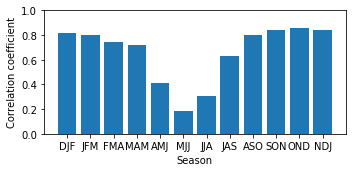
Evaluate the seasonal skill for predicting the ONI
[7]:
from ninolearn.plot.evaluation import plot_correlation
import pandas as pd

# make a plot of the seasonal correaltion
# note: - pd.tseries.offsets.MonthBegin(1) appears to ensure that the correlations are plotted
# agains the correct season

plot_correlation(oni.loc[testtimey[0]: testtimey[-1]], pred_oni, testtimey - pd.tseries.offsets.MonthBegin(1), title="")

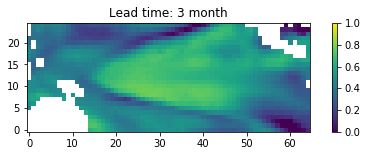
Check the correlations on a map
In the following the pearson correlation coefficent between the predicted and the observed value for each grid point are computed and afterwards plotted.
[8]:
# rehshape predictions to a map
corr_map = np.zeros(pred.shape[1])

for j in range(len(corr_map)):
    corr_map[j] = np.corrcoef(pred[:,j], test_label[:,j])[0,1]
corr_map = corr_map.reshape((label.shape[1:]))
[9]:
%matplotlib inline
# Plot correlation map
fig, ax = plt.subplots(figsize=(8,2))
plt.title(f"Lead time: {lead} month")
C=ax.imshow(corr_map, origin='lower', vmin=0, vmax=1)
cb=plt.colorbar(C)

Animate the full test prediction
[12]:
import matplotlib.animation as animation

def animation_ed(true, pred, nino,  nino_pred, time):
    fig, ax = plt.subplots(3, 1, figsize=(6,7), squeeze=False)

    vmin = -3
    vmax = 3

    true_im = ax[0,0].imshow(true[0], origin='lower', vmin=vmin, vmax=vmax, cmap=plt.cm.bwr)
    pred_im = ax[1,0].imshow(pred[0], origin='lower', vmin=vmin, vmax=vmax, cmap=plt.cm.bwr)
    title = ax[0,0].set_title('')

    ax[2,0].plot(time, nino)
    ax[2,0].plot(time, nino_pred)
    ax[2,0].set_ylim(-3,3)
    ax[2,0].set_xlim(time[0], time[-1])

    vline = ax[2,0].plot([time[0], time[0]], [-10,10], color='k')


    def update(data):
        true_im.set_data(data[0])
        pred_im.set_data(data[1])
        title_str = np.datetime_as_string(data[0].time.values)[:10]
        title.set_text(title_str)

        vline[0].set_data([data[2], data[2]],[-10,10])

    def data_gen():
        k = 0
        kmax = len(true)
        while k<kmax:

            yield true.loc[time[k]], pred.loc[time[k]], time[k]
            k+=1

    ani = animation.FuncAnimation(fig, update, data_gen, interval=100, repeat=True, save_count=len(true))
    plt.close("all")
    return ani
[13]:
from IPython.display import HTML
ani = animation_ed(test_label_map, pred_map,
                   oni.loc[testtimey[0]:testtimey[-1]], pred_oni,
                   testtimey)

HTML(ani.to_html5_video())
[13]:
So it looks like that the Encoder-Decoder ensemble has some skill. However, more research is needed to release the full potential of this model.
Maybe you are interested working on this? :D